library(naniar) # Handling and visualizing missing data
library(ranger) # ranger包用于随机森林等相关操作
library(tidymodels) # 用于建模流程的框架
tidymodels_prefer()
theme_set(theme_bw())3 缺失值处理
处理缺失值是数据分析中的重要环节。常见的缺失值处理方法包括:
部分模型对缺失值是不敏感的,换句话说我们在使用这些模型时可以不处理缺失值,或尝试采用这类模型来规避处理缺失值的步骤。常见的对缺失值不敏感的模型包括:决策树、提升树、随即森林。
- 删除/过滤(Section 3.3):删除含有缺失值的观测。
- 插补(Section 3.4) :使用均值或中位数填补缺失值、使用插值法填补缺失值。
- 编码:将缺失值编码为一个新的类别。
3.1 调查缺失数据
set.seed(383)
scat_split <- initial_split(scat, strata = Species)
scat_tr <- training(scat_split)
scat_te <- testing(scat_split)

scat_rs <- vfold_cv(scat_tr, repeats = 5, strata = Species)
scat_tr_pred <- scat_tr |>
select(-Species)naniar::miss_var_summary(scat_tr_pred)# A tibble: 18 × 3
variable n_miss pct_miss
<chr> <int> <num>
1 Taper 14 17.3
2 TI 14 17.3
3 Diameter 4 4.94
4 d13C 2 2.47
5 d15N 2 2.47
6 CN 2 2.47
7 Mass 1 1.23
8 Month 0 0
9 Year 0 0
10 Site 0 0
11 Location 0 0
12 Age 0 0
13 Number 0 0
14 Length 0 0
15 ropey 0 0
16 segmented 0 0
17 flat 0 0
18 scrape 0 0 # 创建存在缺失值和不存在缺失值的列向量
miss_cols <- c("Taper", "TI", "Diameter", "Mass", "d13C", "d15N", "CN")
non_miss_cols <- c(
"Month",
"Year",
"Site",
"Location",
"Age",
"Number",
"Length",
"ropey",
"segmented",
"flat",
"scrape"
)
# 可视化缺失值-upset plot
naniar::gg_miss_upset(scat_tr_pred, nsets = 10)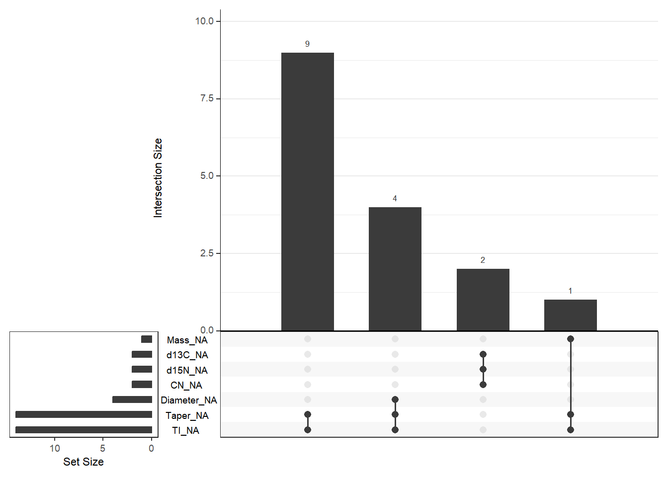
3.2 缺失值出现的原因
理解缺失值出现的原因有助于选择合适的处理方法。缺失值的出现主要由以下3种形式:
- 完全随机缺失(MCAR):缺失值的出现与任何变量无关,完全随机。例如,数据录入错误导致的缺失。
- 随机缺失(MAR):缺失值的出现与其他观测变量有关,但与缺失值本身无关。例如,收入较低的人群更可能不报告其收入。
- 非随机缺失(MNAR):缺失值的出现与缺失值本身有关。例如,患有某种疾病的人更可能不报告其健康状况。
在实际情况中,我们可以参照下表判断缺失值类型并对齐进行处理:
| 缺失值类型 | 核心定义 | 判断依据 | 适用处理方法 | 方法优缺点 | 适用场景 |
|---|---|---|---|---|---|
| 完全随机缺失(MCAR) | 缺失值出现完全随机,与任何变量(包括缺失值本身、其他观测变量)均无关 | 1. 缺失样本在各观测变量上的分布,与完整样本无显著差异; 2. 对任意变量,缺失与否的分组间无统计学差异 |
1. 行删除(删除含缺失的样本); 2. 列删除(删除缺失率过高的变量); 3. 均值/中位数/众数填充 |
优点:操作简单,无额外假设,结果偏差小; 缺点:样本量较小时会导致数据量大幅减少 |
数据录入错误、设备故障导致的随机缺失;缺失率低(通常<5%)的数据集 |
| 随机缺失(MAR) | 缺失值出现与其他观测变量相关,但与缺失值本身的大小无关 | 1. 缺失仅与可观测变量相关,控制这些变量后,缺失随机; 2. 例如“年龄”影响“收入”缺失,但“收入”缺失与否和“实际收入值”无关 |
1. 多重插补(Multiple Imputation); 2. 最大似然估计(Maximum Likelihood); 3. 基于相关变量的回归填充 |
优点:利用已有变量信息,降低偏差,保留更多数据; 缺点:需正确识别相关观测变量,建模过程较复杂 |
调查中特定人群(如高年龄、低学历)对某问题的选择性不回答;缺失率中等(5%-20%)的数据集 |
| 非随机缺失(MNAR) | 缺失值出现与缺失值本身的大小直接相关,存在“自我选择”偏差 | 1. 缺失与缺失值本身相关,无法通过观测变量解释; 2. 例如“高收入者”更可能不填“收入”,“病情严重者”更可能不填“健康评分” |
1. 敏感性分析(评估缺失对结果的影响); 2. 选择模型/模式混合模型(需结合领域假设); 3. 基于专家经验的合理推测填充 |
优点:可在一定程度上处理系统性偏差; 缺点:依赖强假设,结果稳定性差,需谨慎解读 |
涉及隐私、敏感信息(收入、健康、信用)的调查数据;存在明显选择性偏差的数据集 |
3.3 过滤
有两种配方步骤可用于缺失值的过滤:
-
recipe::step_naomit(): 删除有缺失值的行(即删除有缺失值的观测值)。 -
recipe::step_filter_missing(): 删除缺失值超过一定阈值的列(变量)。
na_omit_rec <- recipe(Species ~ ., data = scat_tr) |>
  step_naomit(everything()) |>
  prep()

all_complete <- bake(na_omit_rec, new_data = NULL)
filter_features_rec <-
recipe(Species ~ ., data = scat_tr) |>
step_filter_missing(everything(), threshold = 0.1) |>
prep()
bake(filter_features_rec, new_data = NULL)# A tibble: 81 × 17
Month Year Site Location Age Number Length Diameter Mass d13C d15N
<fct> <int> <fct> <fct> <int> <int> <dbl> <dbl> <dbl> <dbl> <dbl>
1 January 2012 ANNU off_edge 3 7 5.5 21.9 26.4 -27.6 3.89
2 January 2012 ANNU off_edge 5 2 11 17.5 16.2 -28.6 7.34
3 January 2012 ANNU middle 5 1 20.5 18 11.2 -27.4 6.06
4 February 2013 ANNU edge 5 4 10.5 15.5 12.8 -25.8 3.88
5 February 2013 ANNU off_edge 5 4 11.5 17.5 14.1 -27.3 6.61
6 February 2013 ANNU off_edge 5 5 7.5 18 21.7 -27.2 9.07
7 April 2012 YOLA middle 4 4 5.5 21.7 19.2 -29.1 8.72
8 April 2012 YOLA middle 3 1 9 21.6 9.74 -29.8 10.3
9 April 2012 YOLA off_edge 5 2 16.5 18.7 10.2 -28.5 5.59
10 April 2012 ANNU off_edge 4 5 5 13.8 5.5 -27.7 1.84
# ℹ 71 more rows
# ℹ 6 more variables: CN <dbl>, ropey <int>, segmented <int>, flat <int>,
# scrape <int>, Species <fct># use the tody method to determine which were removed
tidy(filter_features_rec, 1)# A tibble: 2 × 2
terms id
<chr> <chr>
1 Taper filter_missing_JiP8Z
2 TI filter_missing_JiP8Z3.4 插补
插补是通过使用已有数据来估计和填补缺失值的过程。recipe中用于预测变量插补的函数包括:recipes::step_impute_bag(), recipes::step_impute_knn(), recipes::step_impute_linear(), recipes::step_impute_lower(), recipes::step_impute_mean(), recipes::step_impute_median(), recipes::step_impute_mode(), recipes::step_impute_roll()。它们各自具体的作用可以从其函数名称中了解(,例如recipes::step_impute_linear()即利用线性回归模型对缺失值进行插补),大致可分为两种类型,基于模型的插补和基于算术统计值的插补。
3.4.1 基于模型的插补
以线性回归模型插补为例,使用变量Age、Length、Number和Location建立线性回归模型,对变量Taper的缺失值进行插补。
linear_impute_rec <-
  recipe(Species ~ ., data = scat_tr) |>
  step_impute_linear(
    Taper,
    impute_with = imp_vars(Age, Length, Number, Location)
  ) |>
  prep()

bake(linear_impute_rec, new_data = NULL) |>
  filter(is.na(Taper)) # 查看插补后的Taper列缺失值数量
# A tibble: 0 × 19
# ℹ 19 variables: Month <fct>, Year <int>, Site <fct>, Location <fct>,
# Age <int>, Number <int>, Length <dbl>, Diameter <dbl>, Taper <dbl>,
# TI <dbl>, Mass <dbl>, d13C <dbl>, d15N <dbl>, CN <dbl>, ropey <int>,
# segmented <int>, flat <int>, scrape <int>, Species <fct>tidy(linear_impute_rec, 1) # 查看使用的变量# A tibble: 1 × 3
terms model id
<chr> <list> <chr>
1 Taper <lm> impute_linear_jh0Cw我们可以通过在参数impute_with中传入单独的变量对缺失值进行插补,这样做的好处是可以根据传入变量的分组对缺失值的插补实现差异化处理。
linear_impute_rec_group <-
  recipe(Species ~ ., data = scat_tr) |>
  step_mutate(Taper_missing = is.na(Taper)) |>
  step_impute_linear(Taper, impute_with = imp_vars(Location)) |>
  prep()

bake(linear_impute_rec_group, new_data = NULL) |>
  filter(Taper_missing) |>
  count(Taper, Location)
# A tibble: 3 × 3
Taper Location n
<dbl> <fct> <int>
1 24.2 middle 10
2 29.9 edge 2
3 30.5 off_edge 2